Magnetic coordinates and fields#

Computing magnetic field coordinates#

The following routines compute magnetic coordinates for a given set of positions. The following coordinates are computed:

McIlwain Lm parameter
Roederer L* parameter
Φ coordinate (Φ=2π Bo/L*)
magnetic field magnitude at the mirror point
magnetic field magnitude at equator
second invariant I parameter
magnetic local time (MLT)

Concerning the Lm and L* parameters, the IRBEM routines outputs also encodes whether local particles are trapped or not - either because they don’t belong to a closed drift shell, or because the drift shell intersects the atmosphere. The coding of this information is presented in the following figure:

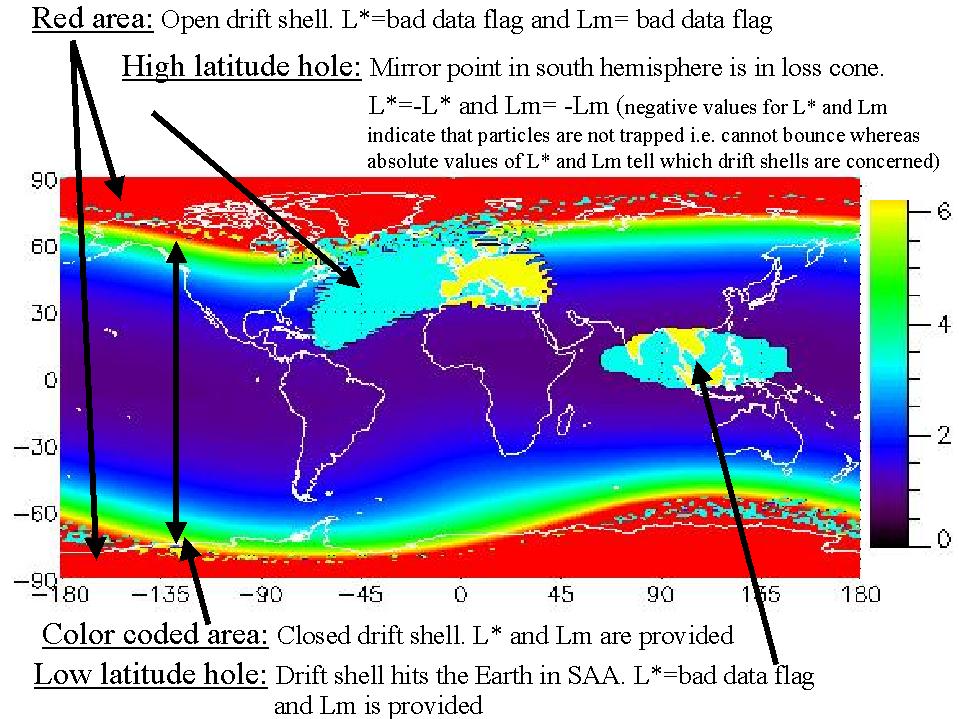
../_images/Lstar.jpg — Coding of the Lm and L* parameters in IRBEM routines#

MAKE_LSTAR#

This function allows one to compute the magnetic coordinates at any spacecraft positions.

A set of internal/external field can be selected.

Note

This routine computes the L* parameter for locally mirroring particles (local picth angle of 90 degrees). See MAKE_LSTAR_SHELL_SPLITTING to compute L* for arbitrary pitch angles.

Note

For a fast approximation of this function for the Olson-Pfitzer Quiet magnetic field model, see the LANDI2LSTAR routine.

Inputs:

ntime (integer) – number of time points
kext (integer) – key for the External magnetic field model
options (array of 5 integer) – IRBEM options
sysaxes (integer) – key for the input coordinate system (see Coordinate systems)
iyear (array of ntime integer) – the year
idoy (array of ntime integer) – the day of year (January 1st is idoy=1)
UT (array of ntime double) – the time in seconds
x1 (array of ntime double) – first coordinate according to sysaxes
x2 (array of ntime double) – second coordinate according to sysaxes
x3 (array of ntime double) – third coordinate according to sysaxes
maginput (array of [25, ntime] double) – Magnetic field inputs

Outputs:

Lm (array of ntime double) – L McIlwain - see Coding of the Lm and L* parameters in IRBEM routines
Lstar (array of ntime double) – Roederer L* or Φ=2π Bo/L* (nT Re²), depending on the options value - for L*, see Coding of the Lm and L* parameters in IRBEM routines
Blocal (array of ntime double) – magnitude of magnetic field at point (nT)
Bmin (array of ntime double) – magnitude of magnetic field at equator (nT)
XJ (array of ntime double) – I, related to second adiabatic invariant (Re)
MLT (array of ntime double) – magnetic local time (h)

Calling sequence:

From MATLAB#

[Lm,Lstar,Blocal,Bmin,J,MLT] = onera_desp_lib_make_lstar(kext,options,sysaxes,matlabd,x1,x2,x3,maginput)

From IDL#

result = call_external(lib_name, 'make_lstar', ntime,kext,options,sysaxes,iyear,idoy,ut, x1,x2,x3, maginput, lm,lstar,blocal,bmin,xj,mlt, /f_value)

From FORTRAN#

call make_lstar1(ntime,kext,options,sysaxes,iyear,idoy,ut, x1,x2,x3, maginput, lm,lstar,blocal,bmin,xj,mlt)

From Python#

model = MagFields()
LLA = {'x1':651, 'x2':63, 'x3':20, 'dateTime':'2015-02-02T06:12:43'}
maginput = {'Kp':40}
output_dictionary = model.make_lstar(LLA, maginput)

MAKE_LSTAR_SHELL_SPLITTING#

This function allows one to compute the magnetic coordinates at any spacecraft position and pitch-angle.

A set of internal/external field can be selected.

Inputs:

ntime (integer) – number of time points
npa (integer) – number of requested pitch angles, up to NALPHA_MAX (see Maximum array sizes)
kext (integer) – key for the External magnetic field model
options (array of 5 integer) – IRBEM options
sysaxes (integer) – key for the input coordinate system (see Coordinate systems)
iyear (array of ntime integer) – the year
idoy (array of ntime integer) – the day of year (January 1st is idoy=1)
UT (array of ntime double) – the time in seconds
x1 (array of ntime double) – first coordinate according to sysaxes
x2 (array of ntime double) – second coordinate according to sysaxes
x3 (array of ntime double) – third coordinate according to sysaxes
alpha (array of npa double) – local pitch angles (deg)
maginput (array of [25, ntime] double) – Magnetic field inputs

Outputs:

Lm (array of [ntime, NALPHA_MAX] double) – L McIlwain - see Coding of the Lm and L* parameters in IRBEM routines
Lstar (array of [ntime, NALPHA_MAX] double) – Roederer L* or Φ=2π Bo/L* (nT Re²), depending on the options value - for L*, see Coding of the Lm and L* parameters in IRBEM routines
Bmirr (array of [ntime, NALPHA_MAX] double) – magnitude of magnetic field at mirror point (nT)
Bmin (array of ntime double) – magnitude of magnetic field at equator (nT)
XJ (array of [ntime, NALPHA_MAX] double) – I, related to second adiabatic invariant (Re)
MLT (array of ntime double) – magnetic local time (h)

Calling sequence:

From MATLAB#

[Lm,Lstar,Bmirror,Bmin,J,MLT] = onera_desp_lib_make_lstar_shell_splitting(kext,options,sysaxes,matlabd,x1,x2,x3,alpha,maginput)

From IDL#

result = call_external(lib_name, 'make_lstar_shell_splitting', ntime,Npa,kext,options,sysaxes,iyear,idoy,ut, x1,x2,x3,alpha,maginput,lm,lstar,bmirr,bmin,xj,mlt, /f_value)

From FORTRAN#

call make_lstar_shell_splitting1(ntime,Npa,kext,options,sysaxes,iyear,idoy,ut, x1,x2,x3, alpha,maginput,lm,lstar,bmirr,bmin,xj,mlt)

LANDI2LSTAR#

This function allows one to compute the magnetic coordinates at any spacecraft positions.

This routine differs from MAKE_LSTAR because L* is deduced from Lm, I and day of year empirically, which is much faster. This is set only for IGRF+Olson-Pfitzer quiet field model (kext can only be 5). The errors in L* values are less than 2%.

Note

This routine computes the L* parameter for locally mirroring particles (local picth angle of 90 degrees). See LANDI2LSTAR_SHELL_SPLITTING to compute L* for arbitrary pitch angles.

Inputs:

ntime (integer) – number of time points
kext (integer) – key for the External magnetic field model
options (array of 5 integer) – IRBEM options
sysaxes (integer) – key for the input coordinate system (see Coordinate systems)
iyear (array of ntime integer) – the year
idoy (array of ntime integer) – the day of year (January 1st is idoy=1)
UT (array of ntime double) – the time in seconds
x1 (array of ntime double) – first coordinate according to sysaxes
x2 (array of ntime double) – second coordinate according to sysaxes
x3 (array of ntime double) – third coordinate according to sysaxes
maginput (array of [25, ntime] double) – Magnetic field inputs

Outputs:

Lm (array of ntime double) – L McIlwain - see Coding of the Lm and L* parameters in IRBEM routines
Lstar (array of ntime double) – Roederer L* or Φ=2π Bo/L* (nT Re²), depending on the options value - for L*, see Coding of the Lm and L* parameters in IRBEM routines
Blocal (array of ntime double) – magnitude of magnetic field at point (nT)
Bmin (array of ntime double) – magnitude of magnetic field at equator (nT)
XJ (array of ntime double) – I, related to second adiabatic invariant (Re)
MLT (array of ntime double) – magnetic local time (h)

Calling sequence:

From MATLAB#

[Lm,Lstar,Blocal,Bmin,J,MLT] = onera_desp_lib_landi2lstar(kext,options,sysaxes,matlabd,x1,x2,x3,maginput)

From IDL#

result = call_external(lib_name, 'landi2lstar', ntime,kext,options,sysaxes,iyear,idoy,ut, x1,x2,x3, maginput, lm,lstar,blocal,bmin,xj,mlt, /f_value)

From FORTRAN#

call landi2lstar1(ntime,kext,options,sysaxes,iyear,idoy,ut, x1,x2,x3, maginput, lm,lstar,blocal,bmin,xj,mlt)

LANDI2LSTAR_SHELL_SPLITTING#

This function allows one to compute the magnetic coordinates at any spacecraft position and pitch-angle.

This routine differs from MAKE_LSTAR_SHELL_SPLITTING because L* is deduced from Lm, I and day of year empirically, which is much faster. This is set only for IGRF+Olson-Pfitzer quiet field model (kext can only be 5). The errors in L* values are less than 2%.

Inputs:

ntime (integer) – number of time points
npa (integer) – number of requested pitch angles, up to NALPHA_MAX (see Maximum array sizes)
kext (integer) – key for the External magnetic field model
options (array of 5 integer) – IRBEM options
sysaxes (integer) – key for the input coordinate system (see Coordinate systems)
iyear (array of ntime integer) – the year
idoy (array of ntime integer) – the day of year (January 1st is idoy=1)
UT (array of ntime double) – the time in seconds
x1 (array of ntime double) – first coordinate according to sysaxes
x2 (array of ntime double) – second coordinate according to sysaxes
x3 (array of ntime double) – third coordinate according to sysaxes
alpha (array of npa double) – local pitch angles (deg)
maginput (array of [25, ntime] double) – Magnetic field inputs

Outputs:

Lm (array of [ntime, NALPHA_MAX] double) – L McIlwain - see Coding of the Lm and L* parameters in IRBEM routines
Lstar (array of [ntime, NALPHA_MAX] double) – Roederer L* or Φ=2π Bo/L* (nT Re²), depending on the options value - for L*, see Coding of the Lm and L* parameters in IRBEM routines
Bmirr (array of [ntime, NALPHA_MAX] double) – magnitude of magnetic field at mirror point (nT)
Bmin (array of ntime double) – magnitude of magnetic field at equator (nT)
XJ (array of [ntime, NALPHA_MAX] double) – I, related to second adiabatic invariant (Re)
MLT (array of ntime double) – magnetic local time (h)

Calling sequence:

From MATLAB#

[Lm,Lstar,Bmirror,Bmin,J,MLT] = onera_desp_lib_landi2lstar_shell_splitting(kext,options,sysaxes,matlabd,x1,x2,x3,alpha,maginput)

From IDL#

result = call_external(lib_name, 'landi2lstar_shell_splitting', ntime,Npa,kext,options,sysaxes,iyear,idoy,ut, x1,x2,x3,alpha,maginput,lm,lstar,blocal,bmin,xj,mlt, /f_value)

From FORTRAN#

call landi2lstar_shell_splitting1(ntime,Npa,kext,options,sysaxes,iyear,idoy,ut, x1,x2,x3, alpha,maginput,lm,lstar,blocal,bmin,xj,mlt)

EMPIRICALLSTAR#

This function allows one to compute L* empirically being given Lm, I and day of year. This is set only for IGRF+Olson-Pfitzer quiet field model (kext can only be 5) so Lm and I provided as input must be computed with this field. The errors in L* values are less than 2%.

Inputs:

ntime (integer) – number of time points
kext (integer) – key for the External magnetic field model
options (array of 5 integer) – IRBEM options
iyear (array of ntime integer) – the year
idoy (array of ntime integer) – the day of year (January 1st is idoy=1)
maginput (array of [25, ntime] double) – Magnetic field inputs
Lm (array of ntime double) – L McIlwain
XJ (array of ntime double) – I, related to second adiabatic invariant (Re)

Outputs:

Lstar (array of ntime double) – L Roederer or Φ=2π Bo/L* (nT Re²), depending on the options value

Calling sequence:

From MATLAB#

Lstar = onera_desp_lib_empiricallstar(kext,options,matlabd,maginput,Lm,J)

From IDL#

result = call_external(lib_name, 'empiricalLstar', ntime,kext,options,iyearsat,idoy, maginput, lm,xj,lstar, /f_value)

From FORTRAN#

call EmpiricalLstar1(ntime,kext,options,iyearsat,idoy,maginput, lm,xj,lstar)

GET_MLT#

Routine to get Magnetic Local Time (MLT) from a GEO position and date.

Inputs:

iyear (integer) – the year
idoy (integer) – the day of year (January 1st is idoy=1)
secs (double) – the time in seconds
xGEO (array of 3 double) – cartesian position in GEO

Outputs:

MLT (double) – Magnetic Local Time (h)

Calling sequence:

From MATLAB#

MLT = onera_desp_lib_get_mlt(matlabd,xGEO)

From IDL#

result = call_external(lib_name, 'get_mlt', iyr,idoy,secs,xGEO,MLT, /f_value)

From FORTRAN#

call get_mlt1(iyr,idoy,secs,xGEO,MLT)

GET_HEMI_MULTI#

This function computes in which magnetic hemisphere is the input location.

Inputs:

ntime (integer) – number of time points
kext (integer) – key for the External magnetic field model
options (array of 5 integer) – IRBEM options
sysaxes (integer) – key for the input coordinate system (see Coordinate systems)
iyear (array of ntime integer) – the year
idoy (array of ntime integer) – the day of year (January 1st is idoy=1)
UT (array of ntime double) – the time in seconds
x1 (array of ntime double) – first coordinate according to sysaxes
x2 (array of ntime double) – second coordinate according to sysaxes
x3 (array of ntime double) – third coordinate according to sysaxes
maginput (array of [25, ntime] double) – Magnetic field inputs

Outputs:

xHEMI (array of ntime integer) – +1 for Northern magnetic hemisphere, -1 for Southern magnetic hemisphere, 0 for invalid magnetic field

Calling sequence:

From MATLAB#

[xHEMI] = onera_desp_lib_get_hemi(kext,options,sysaxes,matlabd,x1,x2,x3,maginput)

From IDL#

result = call_external(lib_name, 'get_hemi_multi_idl',ntime,kext,options,sysaxes,iyear,idoy,ut, x1,x2,x3, maginput,xHEMI,  /f_value)

From FORTRAN#

call GET_HEMI_MULTI(ntime,kext,options,sysaxes,iyear,idoy,ut, x1,x2,x3, maginput,xHEMI)

LSTAR_PHI#

Converts from L* to Φ or vice versa.

Φ=2π*Bo/L*

Inputs:

ntime (integer) – number of time points
whichinv (integer) – direction of the transformation: 1 for L* to Φ, 2 for Φ to L*
options (array of 5 integer) – IRBEM options
iyear (array of ntime integer) – the year
idoy (array of ntime integer) – the day of year (January 1st is idoy=1)

Outputs:

Lstar (array of ntime double) – L* (input or output depending on whichinv value)
Phi (array of ntime double) – Φ (nT Re²,input or output depending on whichinv value)

Calling sequence:

From MATLAB#

out = onera_desp_lib_lstar_phi(which,options,matlabd,in)

From IDL#

result = call_external(lib_name, lstar_phi', ntime,whichinv,options,iyear,idoy,lstar,phi, /f_value)

From FORTRAN#

call lstar_phi1(ntime,whichinv,options,iyear,idoy,lstar,phi)

Points of interest on the field line#

FIND_MIRROR_POINT#

This function finds the magnitude and location of the mirror point along a field line traced from any given location and local pitch-angle for a set of internal/external field to be selected.

Inputs:

kext (integer) – key for the External magnetic field model
options (array of 5 integer) – IRBEM options
sysaxes (integer) – key for the input coordinate system (see Coordinate systems)
iyear (integer) – the year
idoy (integer) – the day of year (January 1st is idoy=1)
UT (double) – the time in seconds
x1 (double) – first coordinate according to sysaxes
x2 (double) – second coordinate according to sysaxes
x3 (double) – third coordinate according to sysaxes
alpha (double) – local pitch-angle (deg)
maginput (array of 25 double) – Magnetic field inputs

Outputs:

Blocal (double) – magnitude of magnetic field at point (nT)
Bmirr (double) – magnitude of the magnetic field at the mirror point (nT)
POSIT (array of 3 double) – GEO coordinates of the mirror point (Re)

Calling sequence:

From MATLAB#

[Blocal,Bmirror,xGEO] = onera_desp_lib_find_mirror_point(kext,options,sysaxes,matlabd,x1,x2,x3,alpha,maginput)

From IDL#

result = call_external(lib_name,  'find_mirror_point', kext,options,sysaxes,iyear,idoy,ut, x1,x2,x3,alpha,maginput, blocal,bmir,posit, /f_value)

From FORTRAN#

call find_mirror_point1(kext,options,sysaxes,iyear,idoy,ut, x1,x2,x3,alpha, maginput,blocal,bmir,posit)

From Python#

model = MagFields()
LLA = {'x1':651, 'x2':63, 'x3':20, 'dateTime':'2015-02-02T06:12:43'}
maginput = {'Kp':40}
alpha = 90
output_dictionary = model.find_mirror_point(LLA, maginput, alpha)

FIND_MAGEQUATOR#

This function finds the GEO coordinates of the magnetic equator along the field line starting from input location for a set of internal/external field to be selected.

Inputs:

kext (integer) – key for the External magnetic field model
options (array of 5 integer) – IRBEM options
sysaxes (integer) – key for the input coordinate system (see Coordinate systems)
iyear (integer) – the year
idoy (integer) – the day of year (January 1st is idoy=1)
UT (double) – the time in seconds
x1 (double) – first coordinate according to sysaxes
x2 (double) – second coordinate according to sysaxes
x3 (double) – third coordinate according to sysaxes
maginput (array of 25 double) – Magnetic field inputs

Outputs:

Bmin (double) – magnitude of magnetic field at equator (nT)
POSIT (array of 3 double) – GEO coordinates of the magnetic equator (Re)

Calling sequence:

From MATLAB#

[Bmin,xGEO] = onera_desp_lib_find_magequator(kext,options,sysaxes,matlabd,x1,x2,x3,maginput)

From IDL#

result = call_external(lib_name, 'find_magequator',  kext,options,sysaxes,iyear,idoy,ut,  x1,x2,x3, maginput, bmin,posit,  /f_value)

From FORTRAN#

call find_magequator1(kext,options,sysaxes,iyear,idoy,ut,  x1,x2,x3, maginput,bmin,posit)

From Python#

model = MagFields()
LLA = {'x1':651, 'x2':63, 'x3':20, 'dateTime':'2015-02-02T06:12:43'}
maginput = {'Kp':40}
alpha = 90
output_dictionary = model.find_magequator(LLA, maginput)

FIND_FOOT_POINT#

This function finds the of the field line crossing a specified altitude in a specified hemisphere for a set of internal/external field to be selected.

Inputs:

kext (integer) – key for the External magnetic field model
options (array of 5 integer) – IRBEM options
sysaxes (integer) – key for the input coordinate system (see Coordinate systems)
iyear (integer) – the year
idoy (integer) – the day of year (January 1st is idoy=1)
UT (double) – the time in seconds
x1 (double) – first coordinate according to sysaxes
x2 (double) – second coordinate according to sysaxes
x3 (double) – third coordinate according to sysaxes
stop_alt (double) – desired altitude of field-line crossing (km)
hemi_flag (integer) – key to select the magnetic hemisphere: * 0 - Same magnetic hemisphere as starting point * +1 - northern magnetic hemisphere * -1 - southern magnetic hemisphere * +2 - opposite magnetic hemisphere from starting point
maginput (array of 25 double) – Magnetic field inputs

Outputs:

XFOOT (array of 3 double) – GDZ coordinates of the foot point (Re)
BFOOT (array of 3 double) – magnetic field vector (GEO) at the foot point (nT)
BFOOTMAG (double) – magnitude of the magnetic field at the foot point (nT)

Calling sequence:

From MATLAB#

[Xfoot,Bfoot,BfootMag] = onera_desp_lib_find_foot_point(kext,options,sysaxes,matlabd,x1,x2,x3,stop_alt,hemi_flag,maginput)

From IDL#

result = call_external(lib_name,  'find_foot_point', kext,options,sysaxes,iyear,idoy,ut, x1,x2,x3,stop_alt,hemi_flag,maginput, xfoot,bfoot,bfootmag, /f_value)

From FORTRAN#

call find_foot_point1(kext,options,sysaxes,iyearsat,idoy,UT,xIN1,xIN2,xIN3,stop_alt,hemi_flag,maginput,XFOOT,BFOOT,BFOOTMAG)

From Python#

model = MagFields()
LLA = {'x1':651, 'x2':63, 'x3':20, 'dateTime':'2015-02-02T06:12:43'}
maginput = {'Kp':40}
stopAlt = 100
hemiFlag = 0
output_dictionary = model.find_foot_point(LLA, maginput, stopAlt, hemiFlag)

Magnetic field computation#

GET_FIELD_MULTI#

This function computes the magnetic field vector (expressed in the GEO coordinate system) at the input locations using the selected internal and external magnetic field models.

Inputs:

ntime (integer) – number of time points
kext (integer) – key for the External magnetic field model
options (array of 5 integer) – IRBEM options
sysaxes (integer) – key for the input coordinate system (see Coordinate systems)
iyear (array of ntime integer) – the year
idoy (array of ntime integer) – the day of year (January 1st is idoy=1)
UT (array of ntime double) – the time in seconds
x1 (array of ntime double) – first coordinate according to sysaxes
x2 (array of ntime double) – second coordinate according to sysaxes
x3 (array of ntime double) – third coordinate according to sysaxes
maginput (array of [25, ntime] double) – Magnetic field inputs

Outputs:

Bgeo (array of [3, ntime] double) – BxGEO, ByGEO, BzGEO of the magnetic field (nT)
Bl (array of ntime double) – magnitude of the magnetic field (nT)

Calling sequence:

From MATLAB#

[Bgeo,B] = onera_desp_lib_get_field(kext,options,sysaxes,matlabd,x1,x2,x3,maginput)

From IDL#

result = call_external(lib_name, 'get_field_multi_idl',ntime,kext,options,sysaxes,iyear,idoy,ut, x1,x2,x3, maginput,Bgeo, Bl,  /f_value)

From FORTRAN#

call GET_FIELD_MULTI(ntime,kext,options,sysaxes,iyear,idoy,ut, x1,x2,x3, maginput,Bgeo,Bl)

From Python#

model = MagFields()
LLA = {'x1':651, 'x2':63, 'x3':20, 'dateTime':'2015-02-02T06:12:43'}
maginput = {'Kp':40}
output_dictionary = model.get_field_multi(LLA, maginput)

GET_BDERIVS#

This function computes the magnetic field and its 1st-order derivatives at each input location for a set of internal/external magnetic field to be selected.

Inputs:

ntime (integer) – number of time points up to NTIME_MAX (see Maximum array sizes)
kext (integer) – key for the External magnetic field model
options (array of 5 integer) – IRBEM options
sysaxes (integer) – key for the input coordinate system (see Coordinate systems)
dX (double) – step size for the numerical derivatives (Re)
iyear (array of ntime integer) – the year
idoy (array of ntime integer) – the day of year (January 1st is idoy=1)
UT (array of ntime double) – the time in seconds
x1 (array of ntime double) – first coordinate according to sysaxes
x2 (array of ntime double) – second coordinate according to sysaxes
x3 (array of ntime double) – third coordinate according to sysaxes
maginput (array of [25, ntime] double) – Magnetic field inputs

Outputs:

Bgeo (array of [3, ntime] double) – BxGEO, ByGEO, BzGEO of the magnetic field (nT)
Bmag (array of ntime double) – magnitude of the magnetic field (nT)
gradBmag (array of [3, ntime] double) – gradients of Bmag in GEO (nT)
diffB (array of [3, 3, ntime] double) – derivatives of the magnetic field vector (nT) for the n^th point, diffB(i,j,n) = dB_i / dx_j

Calling sequence:

From MATLAB#

[Bgeo,B,gradBmag,diffB] = onera_desp_lib_get_bderivs(kext,options,sysaxes,matlabd,x1,x2,x3,maginput)

From IDL#

result = call_external(lib_name, 'get_bderivs_idl',ntime,kext,options,sysaxes,dX,iyear,idoy,ut, x1,x2,x3, maginput,Bgeo,Bmag,gradBmag,diffB,  /f_value)

From FORTRAN#

call GET_BDERIVS(ntime,kext,options,sysaxes,dX,iyear,idoy,ut, x1,x2,x3, maginput,Bgeo,Bmag,gradBmag,diffB)

COMPUTE_GRAD_CURV_CURL#

This function computes gradient and curvature force factors and div/curl of B from the outputs of GET_BDERIVS.

Inputs:

ntime (integer) – number of time points
Bgeo (array of [3, ntime] double) – BxGEO, ByGEO, BzGEO of the magnetic field (nT)
Bmag (array of ntime double) – magnitude of the magnetic field (nT)
gradBmag (array of [3, ntime] double) – gradients of Bmag in GEO (nT)
diffB (array of [3, 3, ntime] double) – derivatives of the magnetic field vector (nT)

Outputs:

grad_par (array of ntime double) – gradient of Bmag along Bgeo (nT/Re)
grad_perp (array of [3, ntime] double) – gradient of Bmag perpendicular to B (nT/Re)
grad_drift (array of [3, ntime] double) – (Bhat x grad_perp)/Bmag, with Bhat=Bgeo/Bmag part of gradient drift velocity (1/Re)
curvature (array of [3, ntime] double) – (Bhat . grad)Bhat, part of curvature force, (1/Re)
Rcurv (array of ntime double) – 1/|curvature|, radius of curvature (Re)
curv_drift (array of [3, ntime] double) – Bhat x curvature, part of curvature drift (1/Re)
curlB (array of [3, ntime] double) – curl of B, part of electrostatic current term (nT/Re)
divB (array of ntime double) – divergence of B, should be zero (nT/Re)

Calling sequence:

From MATLAB#

[grad_par,grad_perp,grad_drift,curvature,Rcurv,curv_drift,curlB,divB] = onera_desp_lib_compute_grad_curv_curl(Bgeo,B,gradBmag,diffB)

From IDL#

result = call_external(lib_name, 'compute_grad_curv_idl',ntime,Bgeo,Bmag,gradBmag,diffB, grad_par,grad_perp,grad_drift,curvature,Rcurv,curv_drift,curlB,divB,   /f_value)

From FORTRAN#

call COMPUTE_GRAD_CURV_CURL(ntime,Bgeo,Bmag,gradBmag,diffB, grad_par,grad_perp,grad_drift,curvature,Rcurv,curv_drift,curlB,divB)

Field tracing#

TRACE_FIELD_LINE#

This function traces a full field line which crosses the input position. The output is a full array of positions of the field line.

Inputs:

kext (integer) – key for the External magnetic field model
options (array of 5 integer) – IRBEM options
sysaxes (integer) – key for the input coordinate system (see Coordinate systems)
iyear (integer) – the year
idoy (integer) – the day of year (January 1st is idoy=1)
UT (double) – the time in seconds
x1 (double) – first coordinate according to sysaxes
x2 (double) – second coordinate according to sysaxes
x3 (double) – third coordinate according to sysaxes
maginput (array of 25 double) – Magnetic field inputs
R0 (double) – radius of the reference surface between which field line is traced (Re)

Outputs:

Lm (double) – L McIlwain
Blocal (array of 3000 double) – magnitude of magnetic field at point (nT)
Bmin (double) – magnitude of magnetic field at equator (nT)
XJ (double) – I, related to second adiabatic invariant (Re)
posit (array of (3, 3000) double) – Cartesian coordinates in GEO along the field line
Nposit (integer) – number of points in posit

Calling sequence:

From MATLAB#

[Lm,Blocal,Bmin,J,POSIT] = onera_desp_lib_trace_field_line(kext,options,sysaxes,matlabd,x1,x2,x3,maginput,R0)

From IDL#

result = call_external(lib_name, 'trace_field_line2',  kext,options,sysaxes,iyear,idoy,ut, x1,x2,x3,maginput,R0,lm,blocal,bmin,xj,posit,Nposit, /f_value)

From FORTRAN#

call trace_field_line2_1(kext,options,sysaxes,iyear,idoy,ut, x1,x2,x3, maginput,R0, lm,blocal,bmin,xj,posit,Nposit)

From Python#

model = MagFields()
LLA = {'x1':651, 'x2':63, 'x3':20, 'dateTime':'2015-02-02T06:12:43'}
maginput = {'Kp':40}
output_dictionary = model.trace_field_line(LLA, maginput)

TRACE_FIELD_LINE_TOWARD_EARTH#

This function traces a field line from the input position to the Earth surface. The output is a full array of positions of the field line, usefull for plotting and visualisation.

Inputs:

kext (integer) – key for the External magnetic field model
options (array of 5 integer) – IRBEM options
sysaxes (integer) – key for the input coordinate system (see Coordinate systems)
iyear (integer) – the year
idoy (integer) – the day of year (January 1st is idoy=1)
UT (double) – the time in seconds
x1 (double) – first coordinate according to sysaxes
x2 (double) – second coordinate according to sysaxes
x3 (double) – third coordinate according to sysaxes
maginput (array of 25 double) – Magnetic field inputs
ds (double) – integration step along the field line (Re)

Outputs:

posit (array of (3, 3000) double) – Cartesian coordinates in GEO along the field line
Nposit (integer) – number of points in posit

Calling sequence:

From MATLAB#

POSIT = onera_desp_lib_trace_field_line_towards_earth(kext,options,sysaxes,matlabd,x1,x2,x3,maginput,ds)

From IDL#

result = call_external(lib_name, 'trace_field_line_towards_earth',  kext,options,sysaxes,iyear,idoy,ut,  x1,x2,x3, maginput, ds,posit,Nposit,  /f_value)

From FORTRAN#

call trace_field_line_towards_earth1(kext,options,sysaxes,iyear,idoy,ut, x1,x2,x3, maginput, ds,posit,Nposit)

DRIFT_BOUNCE_ORBIT#

This function traces a full drift shell for particles that have their mirror point at the input location. The output is a full array of positions of the drift shell, usefull for plotting and visualisation.

Key differences from DRIFT_SHELL :

only positions between mirror points are returned
25 - rather than 48 - azimuths are returned
Lstar accuracy respects options(3) and options(4) (see IRBEM options)
a new parameter R0 is required which specifies the minimum radial distance allowed along the drift path (usually R0 = 1, but use R0 < 1 in the drift loss cone)
hmin and hmin_lon outputs provide the altitude and longitude (in GDZ) of the minimum altitude point along the drift shell (among those traced, not just those returned).

Inputs:

kext (integer) – key for the External magnetic field model
options (array of 5 integer) – IRBEM options
sysaxes (integer) – key for the input coordinate system (see Coordinate systems)
iyear (integer) – the year
idoy (integer) – the day of year (January 1st is idoy=1)
UT (double) – the time in seconds
x1 (double) – first coordinate according to sysaxes
x2 (double) – second coordinate according to sysaxes
x3 (double) – third coordinate according to sysaxes
alpha (double) – pitch angle at input location (deg)
maginput (array of 25 double) – Magnetic field inputs
R0 (double) – radius of the minimum allowed radial distance along the drift orbit (Re)

Outputs:

Lm (double) – L McIlwain
Lstar (double) – L Roederer or Φ=2π Bo/L* (nT Re²), depending on the options value
Blocal (array of (1000, 25) double) – magnitude of magnetic field at point (nT)
Bmin (double) – magnitude of magnetic field at equator (nT)
XJ (double) – I, related to second adiabatic invariant (Re)
posit (array of (3, 1000, 25) double) – Cartesian coordinates in GEO along the drift shell
Nposit (array of 25 integer) – number of points in posit along each traced field line

Calling sequence:

From MATLAB#

[Lm,Lstar,Blocal,Bmin,Bmir,J,POSIT,hmin,hmin_lon] = onera_desp_lib_drift_bounce_orbit(kext,options,sysaxes,matlabd,x1,x2,x3,alpha,maginput,R0)

From IDL#

result = call_external(lib_name, 'drift_bounce_orbit2',  kext,options,sysaxes,iyear,idoy,ut,  x1,x2,x3,alpha, maginput,R0, lm,lstar,blocal,bmin,bmir,xj,posit,Nposit,hmin,hmin_lon,  /f_value)

From FORTRAN#

call drift_bounce_orbit2_1(kext,options,sysaxes,iyear,idoy,ut, x1,x2,x3,alpha, maginput,R0 lm,lstar,blocal,bmin,bmir,xj,posit,Nposit,hmin,hmin_lon)

From Python#

model = MagFields()
LLA = {'x1':651, 'x2':63, 'x3':20, 'dateTime':'2015-02-02T06:12:43'}
maginput = {'Kp':40}
output_dictionary = model.drift_bounce_orbit(LLA, maginput)

DRIFT_SHELL#

Note

To only get the points on the drift-bounce orbit, use DRIFT_BOUNCE_ORBIT.

Inputs:

kext (integer) – key for the External magnetic field model
options (array of 5 integer) – IRBEM options
sysaxes (integer) – key for the input coordinate system (see Coordinate systems)
iyear (integer) – the year
idoy (integer) – the day of year (January 1st is idoy=1)
UT (double) – the time in seconds
x1 (double) – first coordinate according to sysaxes
x2 (double) – second coordinate according to sysaxes
x3 (double) – third coordinate according to sysaxes
maginput (array of 25 double) – Magnetic field inputs

Outputs:

Lm (double) – L McIlwain
Lstar (double) – L Roederer or Φ=2π Bo/L* (nT Re²), depending on the options value
Blocal (array of (1000, 48) double) – magnitude of magnetic field at point (nT)
Bmin (double) – magnitude of magnetic field at equator (nT)
XJ (double) – I, related to second adiabatic invariant (Re)
posit (array of (3, 1000, 48) double) – Cartesian coordinates in GEO along the drift shell
Nposit (array of 48 integer) – number of points in posit along each traced field line

Calling sequence:

From MATLAB#

[Lm,Lstar,Blocal,Bmin,J,POSIT] = onera_desp_lib_drift_shell(kext,options,sysaxes,matlabd,x1,x2,x3,maginput)

From IDL#

result = call_external(lib_name, 'drift_shell',  kext,options,sysaxes,iyear,idoy,ut,  x1,x2,x3, maginput, lm,lstar,blocal,bmin,xj,posit,Nposit,  /f_value)

From FORTRAN#

call drift_shell1(kext,options,sysaxes,iyear,idoy,ut, x1,x2,x3, maginput, lm,lstar,blocal,bmin,xj,posit,Nposit)

From Python#

model = MagFields()
LLA = {'x1':651, 'x2':63, 'x3':20, 'dateTime':'2015-02-02T06:12:43'}
maginput = {'Kp':40}
output_dictionary = model.drift_shell(LLA, maginput)